|
|
|
|
|
|
|
|
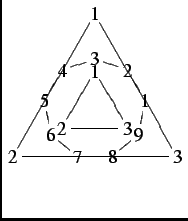
At first three polygons are drawn, a triangle with the edges
![]() , a polygon with 9 edges
, a polygon with 9 edges
![]() and at last a
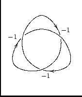
triangle with edges
and at last a
triangle with edges
![]() . Then every knot piece is
placed between 4 edges. In the next example the polygons are made
visible and the numbering of the edges is shown:
. Then every knot piece is
placed between 4 edges. In the next example the polygons are made
visible and the numbering of the edges is shown:
|
|
|
|
Here is the arrangement of the polygons:
|
|
![$\displaystyle \xygraph{
!{0;/r1.0pc/:}
[u]
!{\vover}
!{\vcap-}
[ul]!{\xcaph@(...
...ph@(0)}
} \leftrightarrow
\xygraph{
!{0;/r1.0pc/:} [uu]
!{\xcaph[3]@(0)}
}$](img11.gif)
![$\displaystyle \xygraph{
!{0;/r1.0pc/:}
[u(0.8)]
!{\xcaph@(0)}
!{\vover}
!{\vun...
...0)}
} \leftrightarrow
\xygraph{
!{0;/r1.0pc/:}
[u(0.8)]!{\huncross[2]}
}$](img12.gif)
![$\displaystyle \xygraph{
!{0;/r1.0pc/:}
[u(0.7)]
!{\xoverh[3]}
[ull][ul(0.5)]!{...
...d(0.5)]!{\sbendh@(0)}
[rrrr]!{\sbendv@(0)}
[llllll][u(1.25)]!{\xcaph[-6]@(0)}
}$](img13.gif)
![\xygraph{
!{0;/r2.0pc/:}
!P9''e''{ :{(5,0):} >{}}[u]
!P5''d''{ :{(1.41421,0):...
... {''d3''}{''e5''}{''b4''}{''e5''}}
!{\hcap {''d1''}{''e1''}{''c8''}{''e1''}}
}](img19.gif)
![\xygraph{
!{0;/r2.0pc/:}
!P9''e''{ :{(5,0):} *{\xypolynode} >{-}}[u]
!P5''d''...
...''{ ={45} *{\xypolynode} >{-}}
[ddl][u(0.1)]
!P3''f''{ *{\xypolynode} >{-}}
}](img20.gif)